SIRENA description
Purpose
SIRENA (Software Ifca for Reconstruction of EveNts for Athena X-IFU) is a software package developed to reconstruct the energy of the incoming X-ray photons after their detection in the X-IFU TES detector of the future ESA Athena mission (but it is equally valuable for other TES detectors). This is done by means of two tools called teslib and tesrecons, which are mainly two wrappers to pass a data file to the SIRENA tasks; teslib builds the library with the optimal filters to reconstruct the energies with tesrecons.
Initially, SIRENA was integrated in the SIXTE end-to-end simulations environment, running on simulated data from SIXTE or XIFUSIM (available for the XIFU consortium members upon request at sixte-xifusim@lists.fau.de). Currently, SIRENA is no longer integrated into either SIXTE or XIFUSIM but it continues to process their simulated data and requires the SIXTE software as well as the XIFU instrument files. Similarly, SIRENA can handle real data from laboratory measurements, provided that the data are stored in FITS files in a format compatible with SIRENA.
The SIRENA software is regularly updated and beta versions are often uploaded to a SIRENA GitHub repository.
Files
Auxiliary Files
All the reconstruction methods used by SIRENA software rely on the existence of a library created from a set of data calibration files. In addition, some methods require also a file with the noise data. Let’s describe these auxiliary files in detail.
Noise file
The detector noise file is built by the tool gennoisespec from a a long stream of data. This stream is ingested in gennoisespec, which generates the noise current spectral density, and the weight matrices if it is required, from pulse-free data (removing pulses in case it is necessary).
1) Calibration Stream Simulation
When working with simulated data, the first step is to create a photon list by for example using the SIXTE tool tesgenimpacts which create a piximpact file of zero-energy photons:
> tesgenimpacts PixImpList=noise.piximpact opmode=const tstop=1.0 EConst=0. dtau=1
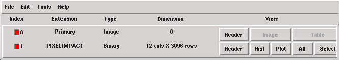
Piximpact file of zero-energy photons.
The second step involves simulating the noise stream, which can be achieved by using the XIFUSIM tool xifusim (:cite:`Kirsch2022`) with the option simnoise=y, simulating fake impacts on the detector based on its physics and generating a noise data stream divided into records:
> xifusim PixImpList=noise.piximpact Streamfile=noise.fits tstop=simulationTime acbias=no\
XMLfilename=myfileXF.xml trig_reclength=10000 simnoise=y
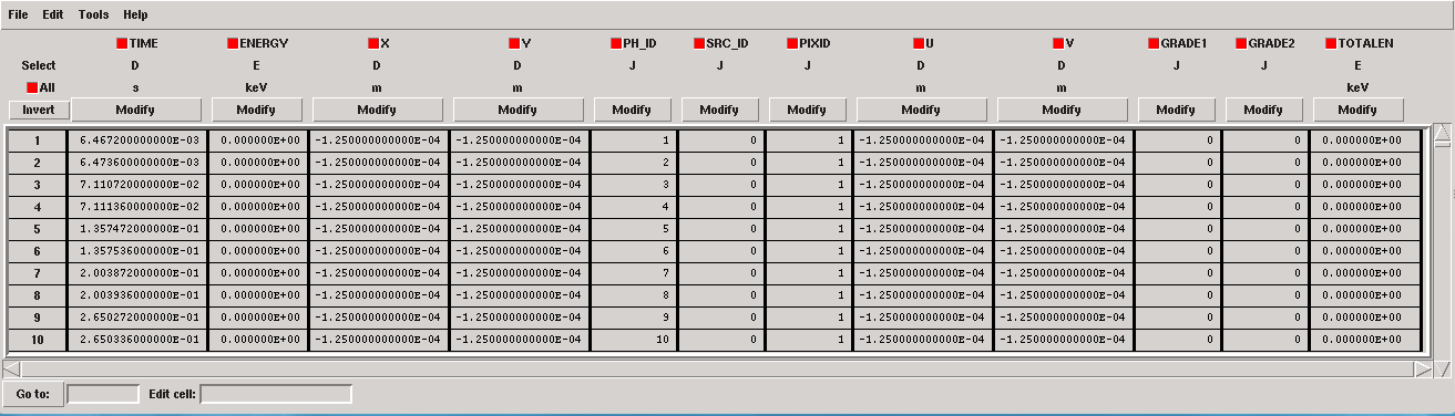
Noise file triggered into records of 10000 samples by using xifusim.
2) Noise spectrum and weight matrices generation
In gennoisespec, data analysis is performed on a per-record basis. When pulses are detected within a record, this tool finds and filters them out, retaining only the pulse-free intervals whose size is determined by the input parameter intervalMinSamples (the hidden input parameter pulse_length further specifies the portion of the record rejected due to a detected pulse). In cases where no pulses are present, the record is divided into pulse-free intervals, the size of which is also controlled by this parameter intervalMinSamples.
Once the pulse-free intervals have been defined, a long noise interval is constructed by aggregating these pulse-free intervals in order to calculate the noise baseline. Additionally, if rmNoiseInterval = yes, the noise intervals with excessively high standard deviation are discarded.
On one hand, the tool computes the FFT of the non-discarded pulse-free intervals (over the unfiltered data) and averages them. Only a specific number of intervals (input parameter nintervals) will be utilized. The noise spectrum density is stored in the NOISE and NOISEALL HDUs in the noise data file.
> gennoisespec inFile=noise.fits outFile=noiseSpec.fits intervalMinSamples=pulseLength \
nintervals=1000 pulse_length=pulseLength

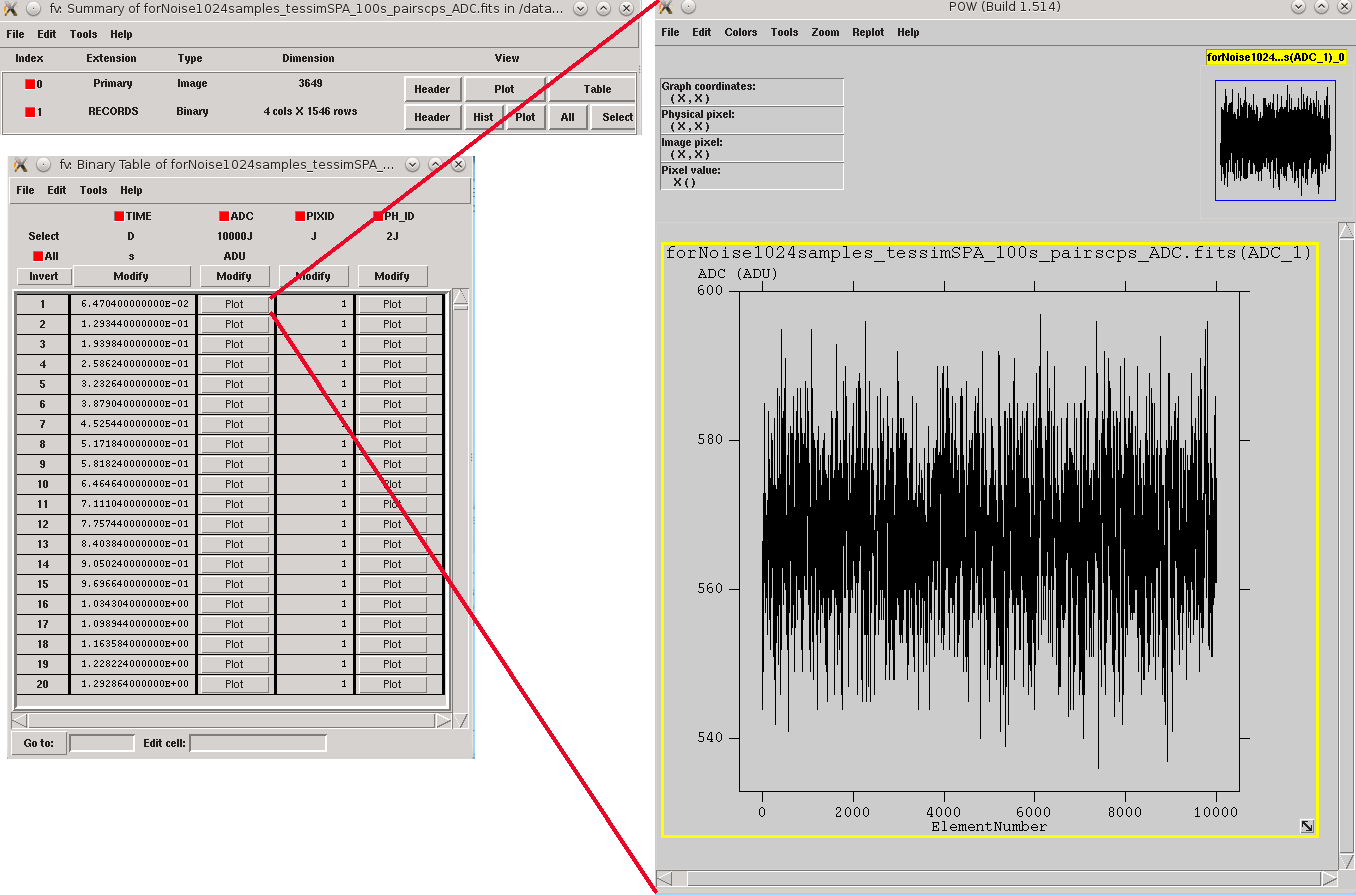
Noise spectrum (see noise file description)
On the other hand, if weightMS = yes the tool calculates the covariance matrix of the noise, \(V^n\), whose elements are expectation values (\(E[·]\)) of two-point products for a pulse-free data sequence \({di}\) (over the unfiltered data) (:cite:`Fowler2015`)
The weight matrix \(W^n\) is the inverse of the covariance matrix, \((V^n)^{-1}\). The weight matrices for different lenghts, Wx, are stored in the WEIGHTMS HDU in the noise data file. The lengths x will be base-2 values and will vary from the base-2 system value closest-lower than or equal-to the intervalMinSamples decreasing until 2.
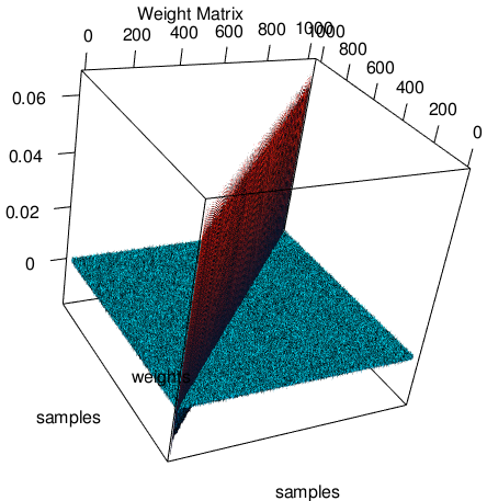
Noise weight matrix (see noise file description)
gennoisespec also adds the BSLN0 and NOISESTD keywords to the NOISE HDU in the noise data file. They store the mean and the standard deviation of the noise (calculated from the long noise interval).
If the noise spectrum or the weight matrices are to be created from a data stream containing pulses, care should be taken with the parameters scaleFactor, samplesUp and nSgms, which are responsible for the detection process.
The sampling rate is calculated using certain keywords in the input FITS file. For tessim simulated data files, tha sampling rate is derived from the DELTAT keyword, where samplingRate=1/deltat. For xifusim simulated data files, each detector type defines a master clock-rate, TCLOCK, and the sampling rate is calculated either from a given decimation factor DEC_FAC (FDM and NOMUX) as samplingRate=1/(tclock·dec_fac), or from the row period P_ROW and the number of rows NUMROW (TDM) as samplingRate=1/(tclock·numrow·p_row). In the case of old simulated files, the sampling rate could be retrieved from the HISTORY keyword in the Primary HDU. If the sampling frequency cannot be obtained from the input file, a message will prompt the user to include the DELTAT keyword (inverse of the sampling rate) in the input FITS file before rerunning the process.
Template Library
The purpose of the library is to store detector pulse magnitudes (templates, covariance matrices, optimal filters…) at different calibration energies, enabling their subsequent use for the reconstruction of input pulses of unknown energy.
To construct this library, a bunch of monochromatic pulses at varying energies are simulated using tesconstpileup (which now generates a piximpact file containing pairs of pulses with constant separation) and either tessim or xifusim (which simulate the detector physics).
1) Calibration Files simulation
The typical run commands to create these calibration files for a given energy monoEkeV and a given (large) separation in samples between the pulses would be as follows
> tesconstpileup PixImpList=calib.piximpact XMLFile=tes.XML timezero=3.E-7\
tstop=simulationTime offset=-1 energy=monoEkeV pulseDistance=separation\
TriggerSize=tsize sample_freq=samplingFreq
where simulationTime should be large enough to simulate around 20000 isolated pulses, and tsize is the size of every simulation stream containing the isolated pulse.
As in the noise simulation, either SIXTE (tessim) or XIFUSIM (xifusim) are suitable for the task.
> tessim PixID=pixelNumber PixImpList=calib.piximpact Streamfile=calib.fits tstart=0. \
tstop=simulationTime triggertype='diff:3:100:suppress' triggerSize=tsize \
PixType=file:mypixel_configuration.fits acbias=yes
where suppress is the time (in samples) after the triggering of an event, during which tessim will avoid triggering again (see figure below).
> xifusim PixImpList=calib.piximpact Streamfile=calib.fits tstart=0. tstop=simulationTime \
XMLfilename=myfileXF.xml trig_reclength=tsize trig_n_pre=PreBufferSize \
trig_n_suppress=suppress acbias=no sample_rate=samplingFreq simnoise=y

Parameters involved in triggering into records from tesconstpileup to tessim and xifusim.
The simulated calibration files are now FITS files with only one HDU called RECORDS [1] populated with four columns: TIME (arrival time of the event), ADC (digitized current), PIXID (pixel identification) and PH_ID (photon identification, for debugging purposes only).
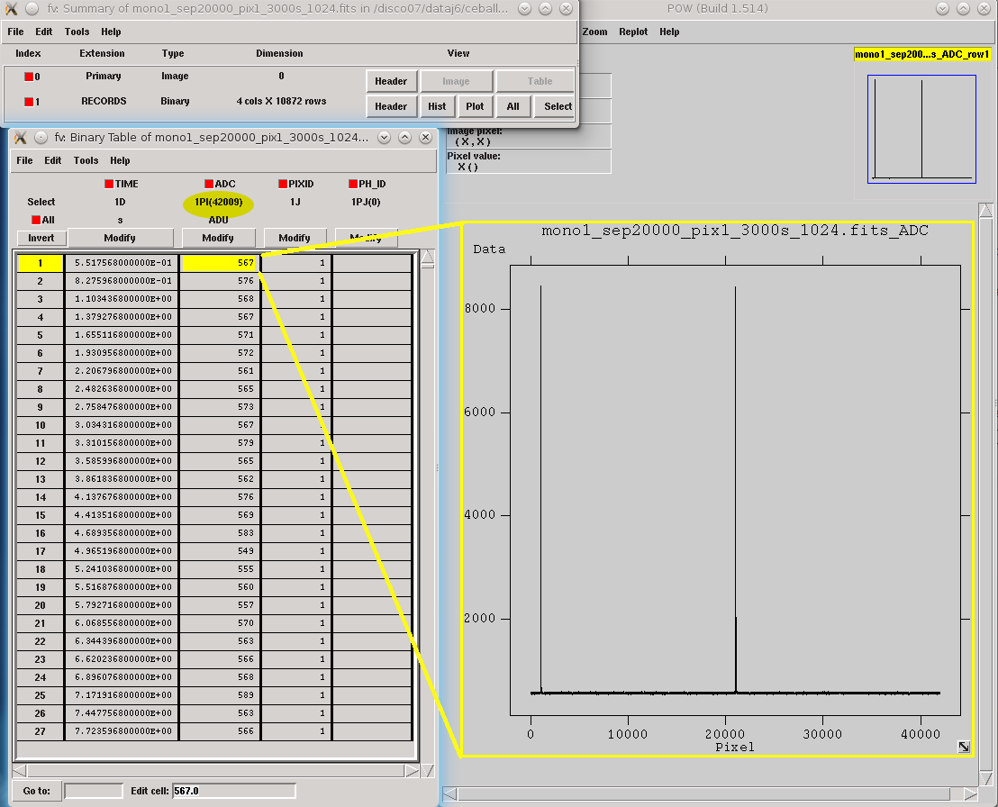
Records in calibration file by using tessim.
2) Library construction
After generating the calibration files for all calibration energies ranging from 1 to N, the library is constructed using the teslib wrapper tool. To execute it with the SIRENA code:
> teslib Recordfile=calib.fits TesEventFile=evtcal.fits largeFilter=8192 \
LibraryFile=library.fits clobber=yes monoenergy=monoEeV_1 EventListSize=1000\
NoiseFile=noiseSpec.fits scaleFactor=sF samplesUp=sU nSgms=nS \
addCOVAR=yes/no addINTCOVAR=yes/no addOFWN=yes/no

[.....]

> teslib Recordfile=calib.fits TesEventFile=evtcal.fits largeFile=8192\
LibraryFile=library.fits clobber=yes monoenergy=monoEeV_N EventListSize=1000\
NoiseFile=noiseSpec.fits scaleFactor=sF samplesUp=sU nSgms=nS \
addCOVAR=yes/no addINTCOVAR=yes/no addOFWN=yes/no
The parameters of teslib for the library creation process are:
RecordFile: record FITS fileTesEventFile: output event list FITS fileLibraryFile: calibration library FITS fileNoiseFile: noise spectrum FITS fileXMLFile: XML input FITS file with instrument definition (ifpreBuffer= yes the library will be built by using filter lengths and their corresponding preBuffer values read from the XML input file)preBuffer: some samples optionally added before the starting time of a pulse (number of added samples read from the XML file)EventListSize: Default size of the event list per recordscaleFactor, samplesUp and nSgms: parameters involved in the pulse detection process
LrsTandLbT: running sum filter length (to get pulse height) and baseline averaging lengthmonoenergy: monochromatic energy of the calibration pulses used to create the current row in the libraryaddCOVAR: add or not pre-calculated values related to COVAR reconstruction method in the library fileaddINTCOVAR: add or not pre-calculated values related to INTCOVAR reconstruction method in the library fileaddOFWN: add or not pre-calculated values related to Optimal Filtering by using Weight Noise matrix in the library filelargeFilter: length (in samples) of the longest fixed filter. If the interval size (intervalMinSamples) used to create the noise exceeds this value, the noise will be decimated accordingly when used to pre-calculate the optimal filters or the covariance matrices. Conversely, if the interval size is shorter, an error will be raisedEnergyMethod: energy calculation Method: OPTFILT (Optimal filtering), 0PAD (0-padding), I2R and I2RFITTED (Linear transformations) (I2R/I2RFITTED are incompatible with
addCOVAR/addINTCOVAR= yes)Ifit: constant to apply the I2RFITTED conversion
FilterMethod:filtering Method: F0 (deleting the zero frequency bin) or B0 (deleting the baseline)intermediateanddetectFile: optionally write intermediate file and name of this intermediate filetstartPulse1andtstartPulse2andtstartPulse3: start time (in samples) of the first, second and third pulse in the record (0 if detection should be performed by the system; greater than 0 if provided by the user)
3) Library structure
The library FITS file comprises 3 HDUs called LIBRARY, FIXFILTT, FIXFILTF which are always present, and 2 HDUs named PRCLCOV and PRCLOFWN which are optional depending on the input parameters addCOVAR and addOFWN.
LIBRARY always includes the following columns:
ENERGY: energies (in eV) in the library
PHEIGHT: pulse heights of the templates
PULSE: templates (obtained by averaging many signals) with baseline. Its length corresponds to the closest lower or equal base-2 value to
largeFilterPULSEB0: baseline-subtracted templates derived from PULSE
MF: matched filters (energy-normalized templates) derived from PULSE
MFB0: baseline-subtracted matched filters derived from MFB0
The number of columns in LIBRARY may increase depending on input parameters or if the library incorporates multiple calibration energies:
PLSMXLFF: long templates according to
largeFilter(obtained by averaging many signals) with baseline. IflargeFilteris a power of 2, it will not appear (only PULSE will be present)
DAB: vectors \(S_{\alpha}- E_{\alpha}(S_{\beta}-S_{\alpha})/(E_{\beta}-E_{\alpha})\), \(d(t)_{\alpha\beta}\) in first order approach. It appears if the library includes multiple calibration energies, not just one
DABMXLFF: DAB according to
largeFilter. IflargeFilteris a power of 2, it will not appear, even if the library includes multiple calibration energiesSAB: vectors \((S_{\beta}-S_{\alpha})/(E_{\beta}-E_{\alpha})\), \(s(t)_{\alpha\beta}\) in first order approach. It appears if the library includes multiple calibration energies, not just one
COVARM: covariance matrices stored in the FITS column as vectors of size pulselength x pulselength. It appears if
addCOVAR= yes oraddINTCOVAR= yesWEIGHTM: weight matrices stored in the FITS column as vectors of size pulselength x pulselength. It appears if
addCOVAR= yes oraddINTCOVAR= yesWAB: matrices \((W_\alpha + W_\beta)/2\) stored as vectors of pulselength x pulselength), being \(\mathit{W}\) weight matrices and \(\alpha\) and \(\beta\) two consecutive energies in the library. It appears if
addCOVAR= yes oraddINTCOVAR= yesTV: vectors \(S_{\beta}-S_{\alpha}\) being \(S_i\) the template at \(\mathit{i}\) energy. It appears if
addINTCOVAR= yestE: scalars \(T \cdot W_{\alpha} \cdot T\). It appears if
addINTCOVAR= yesXM: matrices \((W_\beta + W_\alpha)/t\) stored as vectors of pulselength * pulselength. It appears if
addINTCOVAR= yesYV: vectors \((W_\alpha \cdot T)/t\). It appears if
addINTCOVAR= yesZV: vectors \(\mathit{X \cdot T}\). It appears if
addINTCOVAR= yesrE: scalars \(\mathit{1/(Z \cdot T)}\). It appears if
addINTCOVAR= yes
If preBuffer = yes, the library will be constructed using the filter lengths and their respective preBuffer values extracted from the XML input file. The length of columns PULSE, PULSEB0, MF, MFB0, PAB and DAB will be determined by the maximum filtlen values found in the latest XML files, with filtlen values representing the lengths of filters based on their grading.
The FIXFILTT HDU comprises pre-calculated optimal filters in the time domain for various lengths. These are derived from the matched filters (MF or MFB0 columns) in the Tx columns, or from the SAB column in the ABTx columns. The lengths x are based on values in the binary system and range from the closest lower or equal base-2 system value to the specified largeFilter, gradually decreasing down to 2. Additionally, when largeFilter is not a base-2 value, columns Txmax and ABTxmax are included, where xmax = largeFilter. The FIXFILTT HDU consistently includes Tx columns but ABTx columns are present only if multiple calibration energies (not just one) are incorporated in the library. If preBuffer = yes, the number of Tx columns (or ABTx columns) corresponds to the different grades specified in the XML input file.
The FIXFILTF HDU comprises pre-calculated optimal filters in the frequency domain for various lengths. These are derived from the matched filters (MF or MFB0 columns) in the Fx columns, or from the SAB column in the ABFx columns. The lengths x are based on values in the binary system and range from the closest lower or equal base-2 system value to the specified largeFilter, gradually decreasing down to 2. Additionally, when largeFilter is not a base-2 value, columns Fxmax and ABFxmax are included, where xmax = largeFilter. The FIXFILTF HDU consistently includes Fx columns but ABFx columns are present only if multiple calibration energies (not just one) are incorporated in the library. If preBuffer = yes, the number of Fx columns (or ABFx columns) corresponds to the different grades specified in the XML input file.
The PRCLCOV HDU contains pre-calculated values obtained by utilizing the noise weight matrix derived from the subtraction of the model from pulses for various lengths, PCOVx columns. These lengths x are represented by base-2 values, ranging from the closest lower or equal base-2 system value to the specified largeFilter, gradually decreasing down to 2.
The PRCLOFWN HDU contains pre-calculated values obtained by utilizing the noise weight matrix derived from noise intervals for various lengths, OFWNx columns. These lengths x are represented by base-2 values, ranging from the closest lower or equal base-2 system value to the specified largeFilter, gradually decreasing down to 2.
Input Files
The input data (simulated or laborarory data) files, currently required to be in FITS format, are a sequence of variable length RECORDS, containing at least a column for the TIME of the digitalization process, a column for the detector current (ADC) at these samples, a column for the pixel identification (PIXID) and a column for the photon identification (PH_ID). In the simulated files every record (file row) is the result of an initial triggering process done by the SIXTE simulation tool tessim [2].
Simulated data (pulses) in FITS records by using tessim.
The sampling rate is determined using specific keywords within the input FITS file. For tessim simulated data files, the sampling rate is calculated as samplingRate=1/deltat, where deltat denotes the DELTAT keyword. In the case of xifusim simulated data files, each detector type defines a master clock-rate, TCLOCK; the sampling rate is then calculated either from a given decimation factor, DEC_FAC (for FDM and NOMUX), as samplingRate=1/(tclock·dec_fac), or from the row period, P_ROW, and the number of rows, NUMROW (for TDM), as samplingRate=1/(tclock·numrow·p_row). For older simulated files, the sampling rate could be extracted from the HISTORY keyword in the Primary HDU or from the input XML file. If the sampling frequency cannot be obtained from the input files, a message prompts the user to include the DELTAT keyword (representing the inverse of the sampling rate) in the input FITS file before rerunning the process.
Output Files
The reconstructed energies for all detected events are stored in an output FITS file, controlled by the tesrecons input parameter TesEventFile. Each event is saved in a separate row within the HDU named EVENTS, containing the following information (some of which may only be useful for development purposes):
TIME: arrival time of the event (in s)
SIGNAL: energy of the event (in keV). A post-processing energy calibration is necessary due to the non-linearity of the detector
AVG4SD: average of the first 4 samples of the derivative of the pulse
ELOWRES: energy provided by a low-resolution energy estimator filtered with an 8-sample-length filter (with lags) (in keV). If there is no 8-length filter in the library, ELOWRES=-999.
GRADE1: length of the filter utilized, defined as the distance to the subsequent pulse (in samples), or the pulse length if the next event is beyond this value, or if there are no additional events in the same record
GRADE2: distance to the start time of the preceding pulse (in samples). If the pulse is the first event, this value is fixed to the pulse length
PHI: arrival phase (offset relative to the central point of the parabola) (in samples)
LAGS: number of samples shifted to find the maximum of the parabola
BSLN: mean value of the baseline generally preceding a pulse (according the value in samples of
LbT)RMSBSLN: standard deviation of the baseline generally preceding a pulse (according the value in samples of
LbT)PIXID: pixel number
PH_ID: photon number identification of the first three photons in the respective record for cross-matching with the impact list
GRADING: pulse grade (depending on number of gradings in XML file, in general, VeryHighRes=1, HighRes=2, IntRes=3, MidRes=4, LimRes=5, LowRes=6 and Rejected=-1)
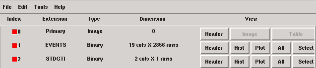
Output event file.
There are additional columns (RISETIME, FALLTIME, RA, DEC, DETX, DETV, SRC_ID, N_XT and E_XT) prepared to potentially store additional information in the future.
In all output files generated by SIRENA (including the noise spectrum file, library file, and reconstructed events file), the keywords CREADATE and SIRENAV indicate the date of file creation and the SIRENA version used execution, respectively.
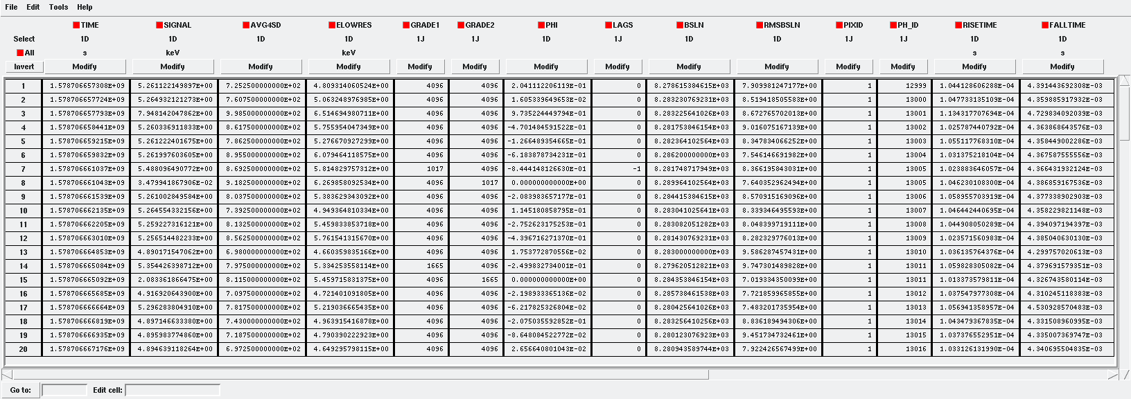
If intermediate = 1, an intermediate FITS file containing useful information (primarily for development purposes) will be created. The intermediate FITS file comprises 2 or 3 HDUs, PULSES, TESTINFO and FILTER. The PULSES HDU inlcudes information about identified pulses: TSTART, I0 (the pulse itself), TEND, QUALITY, TAURISE, TAUFALL and ENERGY. The TESTINFO HDU contains FILDER (the low-pass filtered and differentiated records) and THRESHOLD utilized in detection. If deemed necessary (when OFLib = no or OFLib = yes, filtEeV = 0 and the number of energies in the library FITS file exceeds 1), the FILTER HDU will encompass the optimal filter used for calculating each pulse energy (OPTIMALF or OPTIMALFF column, depending on the time or frequency domain), along with its length (OFLENGTH).
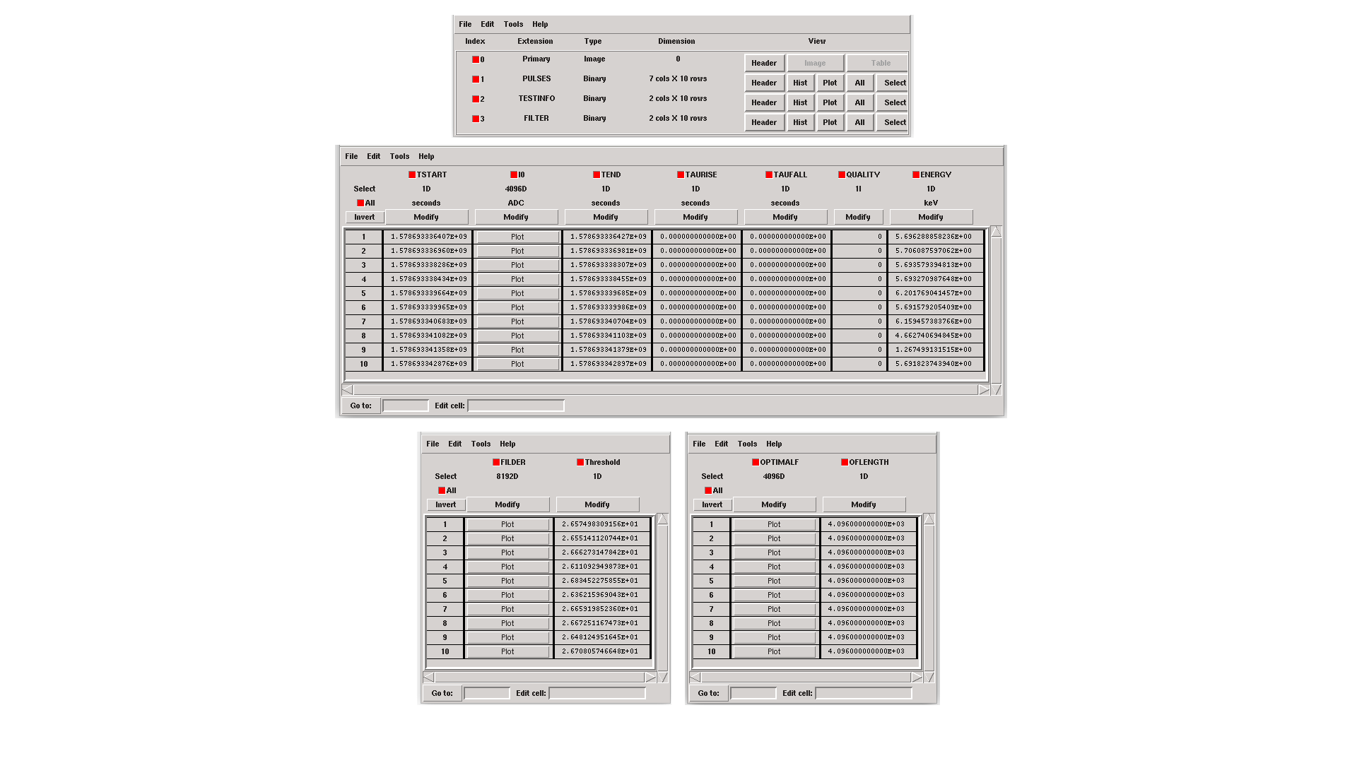
Intermediate output FITS file with extra info.
Reconstruction Process
The energy reconstruction of the input pulse energies is carried out using the tool tesrecons through three main blocks:
Event Detection
Event Grading
Energy Determination
Event Detection
The initial stage of SIRENA processing involves a refined detection process conducted over each RECORD in the input file to identify missing (or secondary) pulses that may overlay the primary (initially triggered) ones. Two algorithms serve this purpose: the Adjusted Derivative (AD) (refer to :cite:`Boyce1999`) and the Single Threshold Crossing (STC) method (implemented in the code to streamline the complexity and computational demands of the AD scheme) (detectionMode).
Adjusted Derivative
The Adjusted Derivative method follows these steps:
1.- The record undergoes differentiation, followed by a median kappa-clipping process where data values exceeding the median plus kappa times the standard deviation of the quiescent signal are iteratively replaced by the median value until no further data points are affected. Subsequently, the threshold is set at the mean value of the clipped data plus nSgms times the standard deviation.
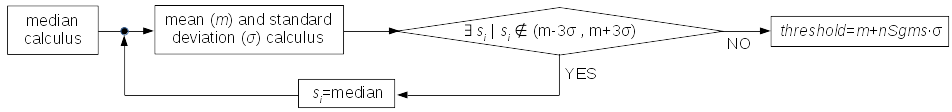
Median kappa-clipping block diagram (at this stage, kappa is hardcoded to 3.).
2.- A pulse is possibly detected whenever the derivarive signal exceeds this threshold.
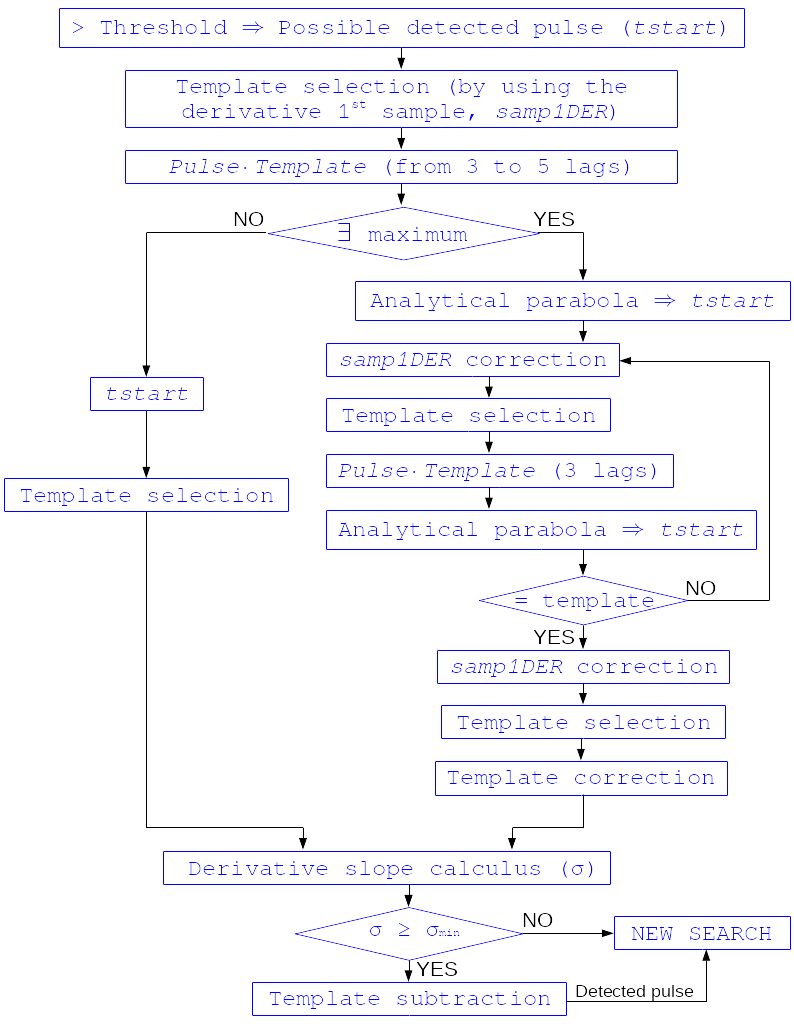
Block diagram illustrating the AD detection process (after threshold establishment).
3.- Based on the first sample of the signal derivative that surpasses the threshold level (samp1DER), a template is chosen from the library. Subsequently, the dot product of the pre-detected pulse and the template is calculated over a span of 25 samples at various positions (lags) around the initial starting time of the pulse to better ascertain its accurate tstarting point. Typically, evaluating the dot product at 3 different lags [3] around the initial detection sample suffices to identify a maximum, and subsequent steps hinge upon whether such a maximum is found or not:
If no maximum of the dot product is detected, the starting time of the pulse is set to the time when the derivative surpasses the threshold (in this scenario, the tstart corresponds to a digitized sample without accounting for potential jitter).
If a maximum of the dot product is identified, a new starting time of the pulse is determined (utilizing the 3-dot-product results around the maximum to analytically define a parabola and locate its apex). Subsequently, an iterative process commences to select the optimal template from the library, yielding a new starting time with each iteration introducing a different level of jitter. Due to jitter, pulses may fall between digitized sample clock intervals, causing the first derivative sample of the pulse itself to deviate from the value of the first sample crossing the threshold, necessitating correction based on the time shift relative to the digitized samples (samp1DER correction).
4.- Each time a sample exceeds the threshold, a check is conducted for the slope of the straight line formed by this sample, its preceding one, and its subsequent one. If the slope is lower than the minimum slope of the templates in the calibration library, the pulse is discarded (as it is likely a residual signal), and a new search is initiated. Conversely, if the slope exceeds the minimum slope of the templates in the calibration library, the pulse is identified as detected.
5.- Once a primary pulse is detected in the record, the system initiates a secondary detection to identify any missing pulses that may be hidden by the primary one. To accomplish this, a model template is selected from the auxiliary library and subtracted at the position of the detected pulse. The first sample of the derivative of the detected pulse (which may differ from the initial one following reallocation performed by the dot product in the previous step) is utilized to once again select the appropriate template from the library. Following the samp1DER correction and accounting for jitter, the 100-sample-long template must be aligned with the pulse before subtraction (template correction). Subsequently, the search for samples exceeding the threshold recommences.
This process iterates until no further pulses are identified.
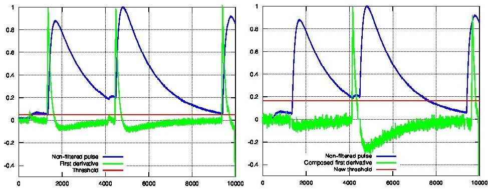
First derivative of initial signal and initial threshold (left) and derivative of signal after subtraction of primary pulses (right).
If the noise level is significant, the input data can undergo low-pass filtering during the initial stage of event detection. This is achieved using the input parameter scaleFactor (\(\mathit{sF}\)). The low-pass filtering is implemented as a box-car function, representing a temporal averaging window. If the cut-off frequency of the filter is \(fc\), the box-car length is calculated as \((1/fc) \times \mathit{samprate}\), where \(\mathit{samprate}\) represents the sampling rate in Hz.
for \(\mathit{sF_1} < \mathit{sF_2}\)
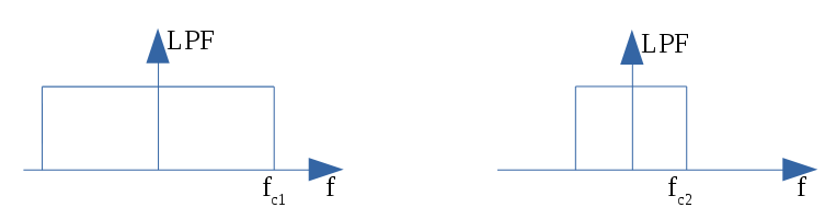
Low-pass filtering (LPF)
If the parameter scaleFactor is too large, the band of the low-pass filter becomes excessively narrow, resulting not only in the rejection of noise during filtering but also in the attenuation of the signal.
Note
To mitigate this issue, an appropriate cut-off frequency for the low-pass filter must be selected to avoid piling-up the first derivative and to detect as many pulses as possible in the input FITS file. However, filtering introduces signal spreading, necessitating a transformation of the start time of the pulse calculated from the first derivative of the low-pass filtered event (which is affected by the filter-induced spreading) into the start time of the non-filtered pulse.
Single Threshold Crossing
1.- This alternative detection method also involves comparing the derivative signal to a threshold (established in the same manner as in the step 1 of the previous algorithm).
2.- If samplesUp consecutive samples of the derivative surpass this threshold, a pulse is detected.
3.- Following detection, the start time of the detected pulse is determined as the first sample of the derivative that crosses the threshold.
4.- If samplesDown consecutive samples of the derivative fall below the threshold, the process of searching for a new pulse begins again.
In contrast to applying either of the last two detection algorithms, for testing and debugging purposes, the SIRENA code can be executed in perfect detection mode, omitting the detection stage, provided that simulated pulses (pairs or triplets) are consistently positioned in all the RECORDS. In this scenario, the start sample of the first/second/third pulse in the record is derived from the input parameter(s) tstartPulse1 [4], tstartPulse2, tstartPulse3 (parameters scaleFactor, samplesUp, or nSgms would not be necessary). Currently, subsample pulse rising has not been implemented in the simulations or in the reconstruction code (potentially a subject for future development).
Event Grading
The Event Grading stage assesses the quality of the pulses based on their proximity to other events within the same record.
After detecting the events in a particular record and establishing their start times, grades are assigned to each event, considering the proximity of adjacent pulses. This classification process follows the information provided in the input XMLFile.
Event Energy Determination: methods
Once the input events have been detected and graded, their energy content can be determined. Currently, all events (regardless of their grade) are processed using the same reconstruction method. However, in the future, a different approach could be adopted, such as simplifying the reconstruction for events with lower resolution.
The SIRENA input parameter that controls the applied reconstruction method is EnergyMethod, which can take values of OPTFILT for Optimal Filtering in Current space, 0PAD for 0-padding in Current space, INTCOVAR for Covariance Matrices, COVAR for a first-order approach of the Covariance matrices method, and I2R or I2RFITTED for Optimal Filtering implementation in (quasi)Resistance space. If optimal filtering is employed and OFNoise is set to WEIGHTN, the noise weight matrix from noise intervals is used instead of the noise spectral density (OFNoise is NSD).
Optimal Filtering by using the noise spectral density
This is the baseline standard technique commonly used for processing microcalorimeter data streams. It relies on two main assumptions. Firstly, it assumes that the detector response is linear, meaning that, the pulse shapes remain identical regardless of their energy, and thus, the pulse amplitude serves as the scaling factor from one pulse to another :cite:`Boyce1999`, :cite:`Szym1993`.
In the frequency domain (as noise can be frequency-dependent), the raw data can be expressed as \(D(f) = E \cdot S(f) + N(f)\), where \(S(f)\) represents the normalized model pulse shape (matched filter), \(N(f)\) represents the noise spectrum, and \(E\) is the scalar amplitude for the photon energy.
The second assumption is that the noise is stationary, meaning it does not vary with time. Consequently, the amplitude of each pulse can be estimated by minimizing (in a weighted least-squares sense) the difference between the noisy data and the model pulse shape. This is achieved by minimizing the \(\chi^2\) condition:
In the time domain, the amplitude corresponds to the optimally filtered sum of values within the pulse, expressed as:
where \(of(t)\) is the time domain representation of the optimal filter in the frequency domain
and \(k\) is the normalization factor to yield \(E\) in energy units
Optimal filtering reconstruction can currently be performed in two different implementations: baseline subtraction (B0 in SIRENA wording), where the baseline value (which is read from the BASELINE keyword in the library file and propagated from the noise file) is subtracted from the signal, and frequency bin 0 (F0), where the frequency bin at f=0 Hz is discarded for constructing the optimal filter. Consequentlly, the final filter is effectively zero-summed, resulting in the rejection of the signal baseline (see :cite:`Doriese2009` for a discussion on the effect of this approach on TES energy resolution). This option is controlled by the parameter FilterMethod.
As the X-IFU detector is nonlinear, the energy estimation after applying any filtering method must be transformed to an unbiased estimation by applying a gain scale obtained through the application of the same method to pulse templates at different energies (which is not performed within SIRENA).
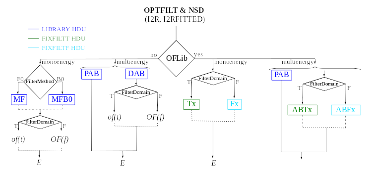
In SIRENA, optimal filters can either be calculated dynamically (on-the-fly) or retrieved as pre-calculated values from the calibration library. This option is determined by the input parameter OFLib. When OFLib = yes, fixed-length pre-calculated optimal filters (Tx or Fx, or ABTx or ABFx) are fetched from the library. The selected length x corresponds to the base-2 system value closest to, but not exceeding, that of the event being reconstructed or largeFilter. Conversely, when OFLib = no, optimal filters are computed specifically for the pulse length of the event being analyzed. The length calculation is governed by the parameter OFStrategy.
When OFStrategy = FREE, the filter length is optimized to the maximum available length (referred to as fltmaxlength), determined by the position of the following pulse or the pulse length if shorter. For OFStrategy = BYGRADE, the filter length is chosen based on the pulse grade (currently read from the XMLFile). Alternatively, for OFStrategy = FIXED, a fixed length (specified by the parameter OFLength) is used for all pulses. These latter two options are primarily intended for testing and development purposes; a typical operational run with on-the-fly calculations employs OFStrategy = FREE. It is important to note that OFStrategy = FREE implicitly sets OFLib = no, while OFStrategy = FIXED or OFStrategy = BYGRADE sets OFLib = yes. Furthermore, when OFLib = no, a noise file must be provided via the parameter NoiseFile, as optimal filters must be computed for each pulse at the required length in this scenario.
In order to reconstruct all events using filters at a single monochromatic energy, the input library should contain only one row with the calibration columns for that specific energy. However, if the input library consists of several monochromatic calibration energies, the optimal filters used in the reconstruction process can be adjusted to the initially estimated energy of the event being analyzed. To achieve this, a first-order expansion of the temporal expression of a pulse at the unknown energy E is taken into account:
where \(b\) represents the baseline level, and \(s(t,E_{\alpha}), s(t,E_{\beta})\) denote pulse templates (PULSEB0 columns) at the corresponding energies \(E_{\alpha}, E_{\beta}\), which encompass the energy \(E\). By rearranging terms, we can further simplify the expression:
then
This expression resembles to the previous one for optimal filtering, where now the data \(d(t)\) is represented by \(d(t,E) - d(t)_{\alpha\beta}\), and the role of the normalized template \(s(t)\) is assumed by \(s(t)_{\alpha\beta}\). Consequently, the optimal filters can be constructed based on \(s(t)_{\alpha\beta}\).
Once more, OFStrategy governs whether the required (interpolated) optimal filter (derived from \(s(t)_{\alpha\beta}\)) is retrieved from the library (at any of the several fixed lengths stored, Fx or Tx if only one energy is included in the library, or ABFx or ABTx if multiple energies are included in the library) or if an appropriate filter is computed dynamically on-the-fly (OFStrategy = FREE).
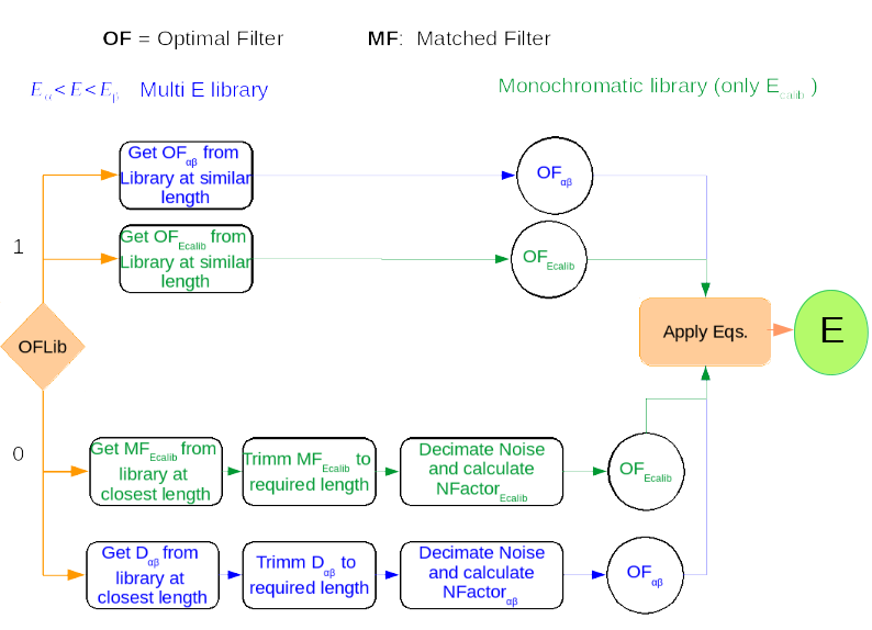
Decision loop for optimal filter calculation
The optimal filtering technique (selected through the input parameter EnergyMethod) can be applied in the frequency or time domain with the option FilterDomain.
The misalignment between the triggered pulse and the template used for the optimal filter can impact the energy estimation. Since the response is highest when the data and the template align, SIRENA incorporates an option to calculate the energy at three predetermined lags between them, aiming for a more accurate estimate than the sampling frequency allows (:cite:`Adams2009`). This feature is controlled by the input parameter LagsOrNot.
Optimal Filtering by using the noise weight matrix from noise intervals
By choosing the input parameter OFNoise as WEIGHTN the optimal filtering method is going to use the noise weight matrix calculated from noise intervals, \(W^n\), rather than the noise spectral density as in the previous section. Using the noise power spectrum (FFT) is also possible, but it introduces an additional wrong assumption of periodicity. The signal-to-noise cost for filtering in the Fourier domain may be small in some cases but it is worth checking the importance of this cost (:cite:`Fowler2017`).
Being \(W^n\) the noise covariance matrix, the best estimate energy is:
where \(M\) is a model matrix whose first column is the pulse shape and the second column is a column of ones in order to calculate the baseline, \(Y\) is the measured data and \(e_1^T \equiv [1, 0]\) is the unit vector to select only the term that corresponds to the energy (amplitude) of the pulse.
Two experimental approaches: adding a preBuffer or 0-padding
In cases where pulses are closer together than the Very High Resolution length, the reconstruction process necessitates the use of shorter optimal filters, resulting in a degradation of the energy resolution, as explored by :cite:`Doriese2009`. To address this issue, two distinct experimental approaches have been devised, namely, variants of Optimal Filtering utilizing the noise spectral density.
a) Adding a preBuffer:
Initially, a few signal samples are added before the triggering point to the pulses template, governed by the parameter preBuffer = yes. These preBuffer values are aligned with the filter length values specified in the XML file, aiding in the construction of the optimal filter.
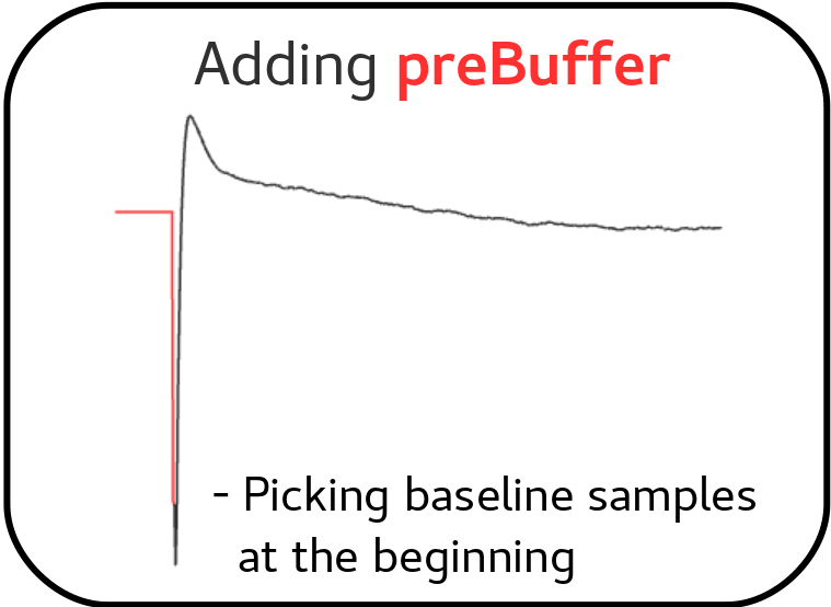
Adding a preBuffer as a variant of Optimal Filtering by using the noise spectral density
b) 0-padding:
Secondly, rather than determining the energy through the scalar product of the short pulse and its corresponding short optimal filter, which is constructed using a template of reduced length, the full filter is consistently utilized. However, in this approach, the full filter, built from a high-resolution-long template, is padded with zeros after the short pulse length. If EnergyMethod = 0PAD, the padding process will be initiated, wherein the filter is padded with zeros from flength_0pad onwards.
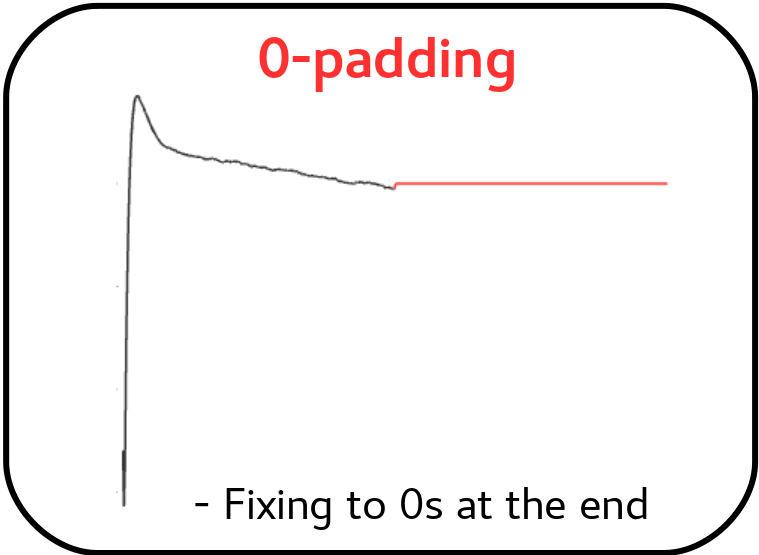
0-padding as a variant of Optimal Filtering by using the noise spectral density
Quasi Resistance Space
A novel approach aimed at dealing with the non-linearity inherent in the signals involves transformating the current signal to a (quasi) resistance space prior the reconstruction process (:cite:`Bandler2006`, :cite:`Lee2015`). This transformation seeks to enhance linearity by mitigating non-linearity arising from the bias circuit, although non-linearity stemming from the Resistance-Temperature transition persists. An additional potential benefit of this approach could be the attainment of a more uniform noise profile across the pulse.
The simulation tool tessim (:cite:`Wilms2016`) is based on a generic model of the TES/absorber pixel featuring a first-stage read-out circuit. The overarching framework of this model is depicted in the figure below. tessim performs the numerical solution of the differential equations governing the time-dependent temperature, \(T(t)\), and current, \(I(t)\), within the TES, as outlined in :cite:`Irwin2005` :
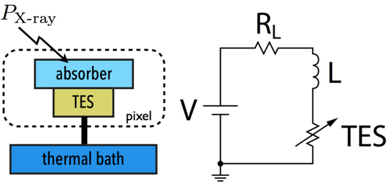
Physics model coupling the thermal and electrical behaviour of the TES/absorber pixel used by tessim.
In the electrical equation, \(L\) is the effective inductance of the readout circuit, \(R_L\) is the effective load resistor and \(V_0\) is the constant voltage bias. Under AC bias conditions,
\(L =\)
LFILTER/TTR²\(R_L =\)
RPARA/TTR²\(\mathit{V0} =\)
I0_START(R0\(+ \mathit{R_L} )\)
and thus the transformation to resistance space would be:
In the aforementioned transformation, the inclusion of a derivative term introduces additional noise, consequently leading to resolution degradation. As a remedy, a new transformation can be implemented by disregarding the circuit inductance ( :cite:`Lee2015` ), effectively suppressing the primary source of non-linearity originating from the first-stage read-out circuit of the detector.
These earlier transformations were previously facilitated by SIRENA. However, SIRENA currently incorporates two transformations accessible through the EnergyMethod command line option. The I2R transformation regards linearization as a linear scale in the height of the pulses concerning energy, whereas the I2RFITTED transformation can also achieve a linear gain scale when reconstructing the signal with a simple filter.
First, let’s examine some definitions provided by columns and keywords in simulated data files to enable the transformation to the (quasi) resistance space:
- ADC:
Data signal in current space [adu (arbitrary data units)] (column)
Group 1:
ADU_CNV:ADU conversion factor [A/adu] (keyword)
I_BIAS:Bias current [A] (keyword)
ADU_BIAS:Bias current [adu] (keyword)
Group 2:
- I0_START:
Bias current [A] (column)
IMIN:Current corresponding to lowest adu value [A] (keyword)
IMAX:Current corresponding to largest adu value [A] (keyword)
I2R transformation
A linearization, in terms of pulse height versus energy, has been incorporated into SIRENA.
If the Group 1 info is available in the input FITS file:
\(I=\)
I_BIAS+ADU_CNV* \((\mathit{ADC}\)-ADU_BIAS\()\)\(\Delta I=\)
ADU_CNV* \((\mathit{ADC}\)-ADU_BIAS\()\)\[\frac{R}{R0} = \mathit{1} - \left(\frac{abs(\Delta I)/\mathit{I\_BIAS}}{1 + abs(\Delta I)/\mathit{I\_BIAS}}\right)\]If the Group 1 information is not available in the input FITS file, Group 2 is utilized. In such instances, the ADU conversion factor must be computed, considering the number of quantification levels (65534):
\(aducnv =\) (
IMAX-IMIN) / 65534\(I = ADC * aducnv\) +
IMIN\(\Delta I= \mathit{I}\) -
I0_STARTI2RFITTED transformation
Looking for a straightforward transformation that would also yield a linear gain scale, a new transformation I2RFITTED was proposed in :cite:`Peille2016`.
\[\frac{R}{V0} \backsim \frac{1}{(I_{fit} + ADC)}\]
Covariance matrices
In real detectors, the assumptions of linearity and stationary noise do not hold strictly true. Consequentlly, an alternative approach is necessary when dealing with non-stationary noise and nonlinear detectors. In this method a set of calibration points is established through numerous pulse repetitions (\(S^i\)) at various energies \((\alpha, \beta, ...)\). For these energy points, a pulse model (PULSEB0 column in the library) is derived by averaging the data pulses \((S_m = <S^i>)\). The deviations of these pulses from the data model \((D^i = S^i - M^i)\) are then used to construct a covariance matrix \(V^{ij} = <D^iD^j>\), with the inverse of this covariance matrix serving as the weight matrix ( \(W\) ). It’s worth noting that non-stationary noise is more accurately characterized by a full noise covariance matrix as opposed to a simpler Fourier transform ( :cite:`Fixsen2004` ).
An initial energy estimation of the unknown signal data is adequate for identifying the calibration points that encompass it. Through linear interpolation of the weight matrix and the signal, the optimal energy estimate becomes only dependent on the energies of the embracing calibration points, the unknown signal, and additional parameters that can be pre-calculated using the calibration data (see Eq. 2 in :cite:`Fixsen2004`):
where \(D = U - S_{m,\alpha}\), being \(U\) the unknown data signal (both \(U\) and \(S_{m,\alpha}\) are signals without a baseline, implying that either the baseline is known or remains constant from calibration to measurement time). Certain terms are precomputed using calibration data and incorporated into the library for retrieval during the reconstruction process. In particular: \(T = (S_{\beta} - S_{\alpha})\), \(t = TW_{\alpha}T\), \(X = (W_{\beta} - W_{\alpha})/t\), \(Y = W_{\alpha}T/t\), \(Z = XT\) and \(r = 1(ZT)\).
Energy reconstruction with Covariance Matrices is selected with input option EnergyMethod = INTCOVAR.
Covariance matrices 0(n)
A first order approximation can be used for the Covariance Matrices method from a first order expansion of the pulse expression at a given t:
where \(b\) is the baseline level, and \(s(t,E_{\alpha}), s(t,E_{\beta})\) are pulse templates (column PULSEB0 in the library) at the corresponding energies \(E_{\alpha}, E_{\beta}\) which embrace the unknown energy \(E\).
resembles an equation of condition in matrix notation \(Y = A\cdot X\) that for a \(\chi^2\) problem with the covariance matrices used as weights (\(W=V^{-1}\)):
where \(e_1^T \equiv [1, 0]\) is the unit vector to select only the term that corresponds to the energy (amplitude) of the pulse.
Energy reconstruction with Covariance Matrices 0(n) is selected with input option EnergyMethod = COVAR. If parameter OFLib = yes, some components can be used from the precalculated values at the libraryColumns (PRCLCOV HDU).
Use of library columns in the different reconstruction methods
1) Optimal filtering and NSD
2) Optimal filtering and WEIGHTN

3) Covariance matrices

4) Covariance matrices O(n)

Examples
In the \(\mathit{sixte/scripts/SIRENA}\) directory of the SIXTE environment, users can find a comprenhensive SIRENA tutorial along with a collection of scripts designed to offer a user-friendly introduction to running SIRENA. Addiotionally, various examples are provided to demostrate different use cases of SIRENA:
Full Energy reconstruction utilizing the (F0) optimal filtering algorithm (filters computed on-the-fly) in the current space, including event detection tailored to the detector specifications outlined in the XMLFile:
>tesrecons Recordfile=inputEvents.fits TesEventFile=outputEvents.fits
OFLib=no OFStrategy=FREE samplesUp=3 nSgms=3.5 samplesDown=4\
LibraryFile=libraryMultiE.fits NoiseFile=noise8192samplesADC.fits\
FilterMethod=F0 clobber=yes intermediate=0 EnergyMethod=OPTFILT \
XMLFile=xifu_detector_lpa_75um_AR0.5_pixoffset_mux40_pitch275um.xml
Energy reconstruction employing the (F0) optimal filtering algorithm (filters extracted from the library) in the current space, with known event positions, for the detector described in the XMLFile:
>tesrecons Recordfile=inputEvents.fits TesEventFile=outputEvents.fits \
LibraryFile=libraryMultiE.fits OFLib=yes\
FilterMethod=F0 clobber=yes intermediate=0 EnergyMethod=OPTFILT\
XMLFile=xifu_detector_lpa_75um_AR0.5_pixoffset_mux40_pitch275um.xml
Energy reconstruction utilizing the Covariance matrices algorithm in the current space, with known event positions, for the detector specified in the XMLFile:
>tesrecons Recordfile=inputEvents.fits TesEventFile=outputEvents.fits
LibraryFile=libraryMultiE.fits \
NoiseFile=noise1024samplesADC.fits clobber=yes intermediate=0 \
EnergyMethod=INTCOVAR XMLFile=xifu_detector_lpa_75um_AR0.5_pixoffset_mux40_pitch275um.xml
Energy reconstruction employing the (F0) optimal filtering algorithm in the I2R Resistance space, with known event positions, for the detector described in the XMLFile, with filters calculated for each event:
>tesrecons Recordfile=inputEvents.fits TesEventFile=outputEvents.fits \
LibraryFile=libraryMultiE.fits \
NoiseFile=noise8192samplesR.fits FilterMethod=F0 clobber=yes intermediate=0 \
EnergyMethod=I2R XMLFile=xifu_detector_hex_baseline.xml OFLib=no OFStrategy=FREE